Load packages and data
##
## Attaching package: 'dplyr'
## The following objects are masked from 'package:stats':
##
##     filter, lag
## The following objects are masked from 'package:base':
##
##     intersect, setdiff, setequal, union
library(tidyr)
library(limma)
library(splines)
library(MSMICA)

# this is the working directory for the case study
setwd('/Users/james/Desktop/Emory University - Ph.D./PhD dissertation/MSMICA/Publication/Abstract/MSMICA_package/MSMICA/vignettes')

# import feature table data
## hilic positive data
data(feature_table_exp_hilicpos)
print(feature_table_exp_hilicpos)
## # A tibble: 11,267 × 44
##       mz  time NM5_GS_0_1 NM5_GS_0_3 NM5_GS_0_5 TM5_GS_0_1 TM5_GS_0_3 TM5_GS_0_5
##    <dbl> <dbl>      <dbl>      <dbl>      <dbl>      <dbl>      <dbl>      <dbl>
##  1  85.0  49.4  127294848   93929747   66033558  159310776   99288246   82335881
##  2  85.0  83.4    9282517   14636989   12921267    8682974   10271317    7132031
##  3  85.1 109.    13329008   15703815    8642594    8449978    8644413    3355450
##  4  85.2  30.8          0   26889920   32196356   25253361   47516277   54826651
##  5  85.3  31.5          0    8566404   14599669    9787948   14132846   23874217
##  6  85.4  30.2          0   13508765   16721105   61654938    9957638    3201424
##  7  85.4  33.8   15066696          0          0   11540798   20251857   31230557
##  8  85.6 156.     6775208    4078654          0    2803849     107620          0
##  9  85.6  76.0          0          0          0    4678248    3290240    1366488
## 10  85.8 106.           0   69397733          0          0          0          0
## # ℹ 11,257 more rows
## # ℹ 36 more variables: NM11_GS_0_1 <dbl>, NM11_GS_0_3 <dbl>, NM11_GS_0_5 <dbl>,
## #   TM11_GS_0_1 <dbl>, TM11_GS_0_3 <dbl>, TM11_GS_0_5 <dbl>, NM6_GS_0_1 <dbl>,
## #   NM6_GS_0_3 <dbl>, NM6_GS_0_5 <dbl>, TM4_GS_0_1 <dbl>, TM4_GS_0_3 <dbl>,
## #   TM4_GS_0_5 <dbl>, NM4_GS_0_1 <dbl>, NM4_GS_0_3 <dbl>, NM4_GS_0_5 <dbl>,
## #   TM6_GS_0_1 <dbl>, TM6_GS_0_3 <dbl>, TM6_GS_0_5 <dbl>, NM7_GS_0_1 <dbl>,
## #   NM7_GS_0_3 <dbl>, NM7_GS_0_5 <dbl>, NM9_GS_0_1 <dbl>, NM9_GS_0_3 <dbl>, …
## c18 negative data
data(feature_table_exp_c18neg)
print(feature_table_exp_c18neg)
## # A tibble: 8,456 × 44
##       mz  time NM5_GS_0_2 NM5_GS_0_4 NM5_GS_0_6 TM5_GS_0_2 TM5_GS_0_4 TM5_GS_0_6
##    <dbl> <dbl>      <dbl>      <dbl>      <dbl>      <dbl>      <dbl>      <dbl>
##  1  85.0 123.     3451142   17675474    4332024    8899759   12204896   12666665
##  2  85.0 288.     2267915    3117932    3828736    4224009    4200063    3788690
##  3  85.0 293.     3691321    2391226    3155868    2361909    4033037    2426635
##  4  85.0  24.9   38858050   43782168   32818312   36913236   36235779   28511185
##  5  85.0  95.0    3104800    2580525    3767773    2646283    2663336    1084595
##  6  85.4 236.     6096726    4051104    1465424    5114500     971445    2515400
##  7  85.5  22.0          0          0          0          0          0          0
##  8  85.5 210.           0    2349999    5895828    1703156    3593730    8463200
##  9  85.6 211.           0     258962    2349208          0    1626943    3316184
## 10  85.7 217.      747185    3036484    5062762    4169043    3809372    9121575
## # ℹ 8,446 more rows
## # ℹ 36 more variables: NM11_GS_0_2 <dbl>, NM11_GS_0_4 <dbl>, NM11_GS_0_6 <dbl>,
## #   TM11_GS_0_2 <dbl>, TM11_GS_0_4 <dbl>, TM11_GS_0_6 <dbl>, NM6_GS_0_2 <dbl>,
## #   NM6_GS_0_4 <dbl>, NM6_GS_0_6 <dbl>, TM4_GS_0_2 <dbl>, TM4_GS_0_4 <dbl>,
## #   TM4_GS_0_6 <dbl>, NM4_GS_0_2 <dbl>, NM4_GS_0_4 <dbl>, NM4_GS_0_6 <dbl>,
## #   TM6_GS_0_2 <dbl>, TM6_GS_0_4 <dbl>, TM6_GS_0_6 <dbl>, NM7_GS_0_2 <dbl>,
## #   NM7_GS_0_4 <dbl>, NM7_GS_0_6 <dbl>, NM9_GS_0_2 <dbl>, NM9_GS_0_4 <dbl>, …
# replace all 0 values with NA after column 2
feature_table_exp_hilicpos[, -c(1:2)] = feature_table_exp_hilicpos[, -c(1:2)] %>%
    mutate_all(~na_if(., 0))

# replace all 0 values with NA after column 2
feature_table_exp_c18neg[, -c(1:2)] = feature_table_exp_c18neg[, -c(1:2)] %>%
    mutate_all(~na_if(., 0))

# median summarize the triplicates
df <- feature_table_exp_hilicpos

# Gather the triplicates into a long format
df_long <- df %>%
  pivot_longer(cols = -c(mz, time), names_to = "sample", values_to = "value")

# Extract the base sample name (without the replicate number)
df_long <- df_long %>%
  mutate(sample_base = sub("(_[0-9])$", "", sample))

# Compute the median for each set of triplicates
df_median <- df_long %>%
  group_by(mz, time, sample_base) %>%
  summarize(median_value = median(value), .groups = "drop")

# Pivot back to the wide format
feature_table_exp_hilicpos <- df_median %>%
  pivot_wider(names_from = sample_base, values_from = median_value)

# View the summarized data frame
print(feature_table_exp_hilicpos)
## # A tibble: 11,267 × 16
##       mz  time NM11_GS_0 NM4_GS_0 NM5_GS_0 NM6_GS_0 NM7_GS_0 NM8_GS_0 NM9_GS_0
##    <dbl> <dbl>     <dbl>    <dbl>    <dbl>    <dbl>    <dbl>    <dbl>    <dbl>
##  1  85.0  49.4  91637758 53374857 93929747 47592345 49580672 65890518 24709252
##  2  85.0  83.4  20848423 11877054 12921267 17645801  7985920 17303431 10586069
##  3  85.1 109.   12062332  3298088 13329008  9183408  1647494 15424423 10908045
##  4  85.2  30.8  43116622 24855153       NA  8517991 34448219 29816051 24415023
##  5  85.3  31.5  13212572 10524120       NA       NA 16114654       NA       NA
##  6  85.4  30.2        NA       NA       NA  5593932  9671769       NA 11869357
##  7  85.4  33.8        NA 11456826       NA       NA  8251705       NA       NA
##  8  85.6 156.         NA       NA       NA  2907723       NA       NA       NA
##  9  85.6  76.0        NA       NA       NA       NA       NA  3804028       NA
## 10  85.8 106.         NA       NA       NA       NA       NA       NA       NA
## # ℹ 11,257 more rows
## # ℹ 7 more variables: TM11_GS_0 <dbl>, TM4_GS_0 <dbl>, TM5_GS_0 <dbl>,
## #   TM6_GS_0 <dbl>, TM7_GS_0 <dbl>, TM8_GS_0 <dbl>, TM9_GS_0 <dbl>
# median summarize the triplicates
df <- feature_table_exp_c18neg

# Gather the triplicates into a long format
df_long <- df %>%
  pivot_longer(cols = -c(mz, time), names_to = "sample", values_to = "value")

# Extract the base sample name (without the replicate number)
df_long <- df_long %>%
  mutate(sample_base = sub("(_[0-9])$", "", sample))

# Compute the median for each set of triplicates
df_median <- df_long %>%
  group_by(mz, time, sample_base) %>%
  summarize(median_value = median(value), .groups = "drop")

# Pivot back to the wide format
feature_table_exp_c18neg <- df_median %>%
  pivot_wider(names_from = sample_base, values_from = median_value)

# View the summarized data frame
print(feature_table_exp_c18neg)
## # A tibble: 8,456 × 16
##       mz  time NM11_GS_0 NM4_GS_0 NM5_GS_0 NM6_GS_0 NM7_GS_0 NM8_GS_0 NM9_GS_0
##    <dbl> <dbl>     <dbl>    <dbl>    <dbl>    <dbl>    <dbl>    <dbl>    <dbl>
##  1  85.0 123.    7722094 10229284  4332024  5469528  8399260  2175857  1929214
##  2  85.0 288.    4407084  3951785  3117932  3267173  4019103  3336862  3128299
##  3  85.0 293.    2607157  3002005  3155868  1907645  1002345   825507  2679529
##  4  85.0  24.9  64373076 39894574 38858050 35446680 35724755 34192423 33235053
##  5  85.0  95.0   2999487  2543380  3104800  1624592  2369531  4524972  2823455
##  6  85.4 236.    4240866  4900397  4051104  3749169  2528974  2431985  4520111
##  7  85.5  22.0        NA       NA       NA       NA       NA       NA       NA
##  8  85.5 210.    3676008       NA       NA  1146822  4697878  6359702  3184766
##  9  85.6 211.    2509843       NA       NA       NA       NA  2801030       NA
## 10  85.7 217.    4761129  3545481  3036484  1748788  3907803  7352392  3096899
## # ℹ 8,446 more rows
## # ℹ 7 more variables: TM11_GS_0 <dbl>, TM4_GS_0 <dbl>, TM5_GS_0 <dbl>,
## #   TM6_GS_0 <dbl>, TM7_GS_0 <dbl>, TM8_GS_0 <dbl>, TM9_GS_0 <dbl>
# Filter out features appear less than 20% of all samples. The intensity column starts from the 3rd column.
feature_table_exp_hilicpos = QC_filter(x = feature_table_exp_hilicpos, metabolite_start_column = 3, minimum_sample_appear = 0.20)
feature_table_exp_c18neg = QC_filter(x = feature_table_exp_c18neg, metabolite_start_column = 3, minimum_sample_appear = 0.20)

# import MSMICA results
## hilic positive data
hilicpos_MSMICA_identified_metabolites = read_csv("MSMICA_test_hilicpos_MSMICA_identified_metabolites_filtered.csv")
## Rows: 2926 Columns: 73
## ── Column specification ────────────────────────────────────────────────────────
## Delimiter: ","
## chr (19): mz_time, Adduct, Name, identification_type, identification_method,...
## dbl (53): mz, time, Probability, metabolite_within_feature_number, time_pred...
## lgl  (1): isomer_exist
##
## ℹ Use `spec()` to retrieve the full column specification for this data.
## ℹ Specify the column types or set `show_col_types = FALSE` to quiet this message.
print(hilicpos_MSMICA_identified_metabolites)
## # A tibble: 2,926 × 73
##       mz  time mz_time    Adduct Name  identification_type identification_method
##    <dbl> <dbl> <chr>      <chr>  <chr> <chr>               <chr>
##  1 348.    284 348.0703_… M+H    AMP   Schymanski level 3a mz matching; retenti…
##  2 385.     90 385.1282_… M+H    S-Ad… Schymanski level 3a mz matching; retenti…
##  3 148.     78 148.0604_… M+H    Glut… Schymanski level 3a mz matching; retenti…
##  4 181.     37 181.072_37 M+H    D-Gl… Schymanski level 3a mz matching; retenti…
##  5  90.1    70 90.055_70  M+H    Alan… Schymanski level 3a mz matching; retenti…
##  6 608.    120 608.0855_… M+H    Urid… Schymanski level 3b mz matching; retenti…
##  7 147.    110 147.1128_… M+H    Lysi… Schymanski level 3a mz matching; retenti…
##  8 134.     83 134.0448_… M+H    Aspa… Schymanski level 3a mz matching; retenti…
##  9 308.    225 308.0909_… M+H    Glut… Schymanski level 3a mz matching; retenti…
## 10 324.     34 324.059_34 M+H    CMP   Schymanski level 3a mz matching; retenti…
## # ℹ 2,916 more rows
## # ℹ 66 more variables: Probability <dbl>,
## #   metabolite_within_feature_number <dbl>, isomer_exist <lgl>,
## #   time_predicted <dbl>, time_difference <dbl>, mean_intensity <dbl>,
## #   PubChem_compound_id <dbl>, HMDB_ID <chr>, KEGG_ID <chr>,
## #   LIPID_MAPS_ID <chr>, ChEBI_ID <dbl>, BioCyc_ID <chr>, DrugBank_ID <chr>,
## #   Mono_mass <dbl>, Formula <chr>, Charge <dbl>, SMILES <chr>, …
## c18 negative data
c18neg_MSMICA_identified_metabolites = read_csv("MSMICA_test_c18neg_MSMICA_identified_metabolites_filtered.csv")
## Rows: 2439 Columns: 73
## ── Column specification ────────────────────────────────────────────────────────
## Delimiter: ","
## chr (19): mz_time, Adduct, Name, identification_type, identification_method,...
## dbl (53): mz, time, Probability, metabolite_within_feature_number, time_pred...
## lgl  (1): isomer_exist
##
## ℹ Use `spec()` to retrieve the full column specification for this data.
## ℹ Specify the column types or set `show_col_types = FALSE` to quiet this message.
print(c18neg_MSMICA_identified_metabolites)
## # A tibble: 2,439 × 73
##       mz  time mz_time    Adduct Name  identification_type identification_method
##    <dbl> <dbl> <chr>      <chr>  <chr> <chr>               <chr>
##  1 662.     20 662.1014_… M-H    NAD   Schymanski level 3a mz matching; retenti…
##  2 664.     20 664.1174_… M-H    NADH  Schymanski level 3a mz matching; retenti…
##  3 742.     20 742.0704_… M-H    NADP  Schymanski level 3a mz matching; retenti…
##  4 426.     22 426.0222_… M-H    ADP   Schymanski level 3a mz matching; retenti…
##  5 766.     20 766.1058_… M-H    Coen… Schymanski level 3a mz matching; retenti…
##  6 784.     20 784.1525_… M-H    FAD   Schymanski level 3a mz matching; retenti…
##  7 346.     21 346.0557_… M-H    AMP   Schymanski level 3a mz matching; retenti…
##  8 383.     27 383.1142_… M-H    S-Ad… Schymanski level 3a mz matching; retenti…
##  9  87.0    24 87.0087_24 M-H    Pyru… Schymanski level 3a mz matching; retenti…
## 10 808.     21 808.1197_… M-H    Acet… Schymanski level 3a mz matching; retenti…
## # ℹ 2,429 more rows
## # ℹ 66 more variables: Probability <dbl>,
## #   metabolite_within_feature_number <dbl>, isomer_exist <lgl>,
## #   time_predicted <dbl>, time_difference <dbl>, mean_intensity <dbl>,
## #   PubChem_compound_id <dbl>, HMDB_ID <chr>, KEGG_ID <chr>,
## #   LIPID_MAPS_ID <chr>, ChEBI_ID <dbl>, BioCyc_ID <chr>, DrugBank_ID <chr>,
## #   Mono_mass <dbl>, Formula <chr>, Charge <dbl>, SMILES <chr>, …
# Prepare the data for MSMICA targeted metabolomics analysis ############################################################################################################

# to make sure there is no duplicate metabolites with the same name but multiple peaks, group by Name and select the metabolites with highest mean intensity
hilicpos_MSMICA_identified_metabolites = hilicpos_MSMICA_identified_metabolites %>%
    group_by(Name) %>%
    slice_max(mean_intensity) %>%
    ungroup()
c18neg_MSMICA_identified_metabolites = c18neg_MSMICA_identified_metabolites %>%
    group_by(Name) %>%
    slice_max(mean_intensity) %>%
    ungroup()

# transpose the table starting at column 32
hilicpos_MSMICA_featuretable_clean_t = t(hilicpos_MSMICA_identified_metabolites[, 32:ncol(hilicpos_MSMICA_identified_metabolites)])
c18neg_MSMICA_featuretable_clean_t = t(c18neg_MSMICA_identified_metabolites[, 32:ncol(c18neg_MSMICA_identified_metabolites)])

# convert the table to a data frame
hilicpos_MSMICA_featuretable_clean_t = as.data.frame(hilicpos_MSMICA_featuretable_clean_t)
c18neg_MSMICA_featuretable_clean_t = as.data.frame(c18neg_MSMICA_featuretable_clean_t)

# set the column names as the Identified_Name
colnames(hilicpos_MSMICA_featuretable_clean_t) = hilicpos_MSMICA_identified_metabolites$Name
colnames(c18neg_MSMICA_featuretable_clean_t) = c18neg_MSMICA_identified_metabolites$Name

# add Group_ID as a column
hilicpos_MSMICA_featuretable_clean_t$Group_ID = rownames(hilicpos_MSMICA_featuretable_clean_t)
c18neg_MSMICA_featuretable_clean_t$Group_ID = rownames(c18neg_MSMICA_featuretable_clean_t)

# move Group_ID as the first column
hilicpos_MSMICA_featuretable_clean_t = tibble(hilicpos_MSMICA_featuretable_clean_t) %>%
    select(Group_ID, everything())
c18neg_MSMICA_featuretable_clean_t = tibble(c18neg_MSMICA_featuretable_clean_t) %>%
    select(Group_ID, everything())

# Seperate the Group_ID into columns: Group, Temperature, Time, SampleID
hilicpos_MSMICA_featuretable_clean_t = hilicpos_MSMICA_featuretable_clean_t %>%
    separate(Group_ID, c("Group", "Temperature", "Time", "Triplicate"), sep = "_") %>%
    # create a new column, sample_tyoe, to indicate the sample type: if Group starts with NM, then it is normal, otherwise it is cancer
    mutate(sample_type = ifelse(stringr::str_detect(Group, "^NM"), "normal", "cancer")) %>%
    # move sample type to the first column
    select(sample_type, everything())
c18neg_MSMICA_featuretable_clean_t = c18neg_MSMICA_featuretable_clean_t %>%
    separate(Group_ID, c("Group", "Temperature", "Time", "Triplicate"), sep = "_") %>%
    # create a new column, sample_tyoe, to indicate the sample type: if Group starts with NM, then it is normal, otherwise it is cancer
    mutate(sample_type = ifelse(stringr::str_detect(Group, "^NM"), "normal", "cancer")) %>%
    # move sample type to the first column
    select(sample_type, everything())

# separate the Group column into Group and ParticipantID: the first two characters are Group, the rest are ParticipantID
hilicpos_MSMICA_featuretable_clean_t = hilicpos_MSMICA_featuretable_clean_t %>%
    separate(Group, c("Group", "ParticipantID"), sep = 2)
c18neg_MSMICA_featuretable_clean_t = c18neg_MSMICA_featuretable_clean_t %>%
    separate(Group, c("Group", "ParticipantID"), sep = 2)

# Convert all intensity values to log2
hilicpos_MSMICA_featuretable_clean_t[, -c(1:6)] = hilicpos_MSMICA_featuretable_clean_t[, -c(1:6)] %>%
    mutate_all(~log2(.))
c18neg_MSMICA_featuretable_clean_t[, -c(1:6)] = c18neg_MSMICA_featuretable_clean_t[, -c(1:6)] %>%
    mutate_all(~log2(.))

# check the data ready for MSMICA targeted metabolomics analysis
print(hilicpos_MSMICA_featuretable_clean_t)
## # A tibble: 42 × 2,929
##    sample_type Group ParticipantID Temperature Time  Triplicate
##    <chr>       <chr> <chr>         <chr>       <chr> <chr>
##  1 normal      NM    5             GS          0     1
##  2 normal      NM    5             GS          0     3
##  3 normal      NM    5             GS          0     5
##  4 cancer      TM    5             GS          0     1
##  5 cancer      TM    5             GS          0     3
##  6 cancer      TM    5             GS          0     5
##  7 normal      NM    11            GS          0     1
##  8 normal      NM    11            GS          0     3
##  9 normal      NM    11            GS          0     5
## 10 cancer      TM    11            GS          0     1
## # ℹ 32 more rows
## # ℹ 2,923 more variables:
## #   `((2-Amino-3-((2-amino-3-((carboxymethyl)amino)-3-oxopropyl)dithio)propanoyl)amino)acetic acid` <dbl>,
## #   `(+)-3-Methoxymorphinan` <dbl>, `(+)-Bornyl-diphosphate` <dbl>,
## #   `(+)-Calycanthidine` <dbl>, `(+)-Chebulic acid` <dbl>,
## #   `(+)-Dukunolide D` <dbl>, `(+)-Luguine` <dbl>,
## #   `(+-)-3-Methyladipic acid` <dbl>, `(+-)-Asarinol B` <dbl>, …
print(c18neg_MSMICA_featuretable_clean_t)
## # A tibble: 42 × 2,445
##    sample_type Group ParticipantID Temperature Time  Triplicate
##    <chr>       <chr> <chr>         <chr>       <chr> <chr>
##  1 normal      NM    5             GS          0     2
##  2 normal      NM    5             GS          0     4
##  3 normal      NM    5             GS          0     6
##  4 cancer      TM    5             GS          0     2
##  5 cancer      TM    5             GS          0     4
##  6 cancer      TM    5             GS          0     6
##  7 normal      NM    11            GS          0     2
##  8 normal      NM    11            GS          0     4
##  9 normal      NM    11            GS          0     6
## 10 cancer      TM    11            GS          0     2
## # ℹ 32 more rows
## # ℹ 2,439 more variables:
## #   `(+)-(3S,4R)-3,4-dihydroxy-3,4-dihydrofluorene` <dbl>,
## #   `(+)-8'-Hydroxyabscisic acid` <dbl>, `(+)-Calycanthidine` <dbl>,
## #   `(+)-Eudesmin` <dbl>, `(+)-Plicamine` <dbl>, `(+)-Prosopinine` <dbl>,
## #   `(+)-Soyacerebroside I` <dbl>, `(+-)-3-Methyladipic acid` <dbl>,
## #   `(-)-2-Aminobutyric acid` <dbl>, `(-)-trans-Carveol glucoside` <dbl>, …
# save the results as a csv file
write.csv(hilicpos_MSMICA_featuretable_clean_t, "MSMICA targeted metabolomics analysis/hilicpos_MSMICA_featuretable_clean_transposed.csv", row.names = FALSE)
write.csv(c18neg_MSMICA_featuretable_clean_t, "MSMICA targeted metabolomics analysis/c18neg_MSMICA_featuretable_clean_transposed.csv", row.names = FALSE)
############################# limma paired t-test #############################
# Factorize the samples into normal and cancer
Group_hilicpos = factor(hilicpos_MSMICA_featuretable_clean_t$sample_type, levels = c("normal", "cancer"))
Group_c18neg = factor(c18neg_MSMICA_featuretable_clean_t$sample_type, levels = c("normal", "cancer"))

# Factorize the ParticipantID
ParticipantID_hilicpos = factor(hilicpos_MSMICA_featuretable_clean_t$ParticipantID)
ParticipantID_c18neg = factor(c18neg_MSMICA_featuretable_clean_t$ParticipantID)

# Create the design matrix
design_T_hilicpos <- model.matrix(~ ParticipantID_hilicpos+Group_hilicpos)
design_T_c18neg <- model.matrix(~ ParticipantID_c18neg+Group_c18neg)

# Extract the intensity values for the limma analysis
hilicpos_intensity = hilicpos_MSMICA_featuretable_clean_t[, 7:ncol(hilicpos_MSMICA_featuretable_clean_t)]
c18neg_intensity = c18neg_MSMICA_featuretable_clean_t[, 7:ncol(c18neg_MSMICA_featuretable_clean_t)]
hilicpos_intensity = as.data.frame(hilicpos_intensity)
c18neg_intensity = as.data.frame(c18neg_intensity)

# transpose the metabolite intensity data
y_T_hilicpos = t(hilicpos_intensity)
y_T_c18neg = t(c18neg_intensity)

# Fit the linear model
fit_hilicpos = lmFit(y_T_hilicpos, design_T_hilicpos)
## Warning: Partial NA coefficients for 255 probe(s)
fit_c18neg = lmFit(y_T_c18neg, design_T_c18neg)
## Warning: Partial NA coefficients for 174 probe(s)
fit2_hilicpos <- eBayes(fit_hilicpos)
fit2_c18neg <- eBayes(fit_c18neg)

# Extract all relevant values from the limma output
limma_outcome_hilicpos = tibble(
    Cancer_log2FC = c(fit2_hilicpos$coefficients[, "Group_hilicposcancer"]),
    t_statistic = c(fit2_hilicpos$t[, "Group_hilicposcancer"]),
    p = c(fit2_hilicpos$p.value[, "Group_hilicposcancer"]))

limma_outcome_c18neg = tibble(
    Cancer_log2FC = c(fit2_c18neg$coefficients[, "Group_c18negcancer"]),
    t_statistic = c(fit2_c18neg$t[, "Group_c18negcancer"]),
    p = c(fit2_c18neg$p.value[, "Group_c18negcancer"]))

limma_outcome_hilicpos$p.fdr = p.adjust(limma_outcome_hilicpos$p, method="BH")
limma_outcome_c18neg$p.fdr = p.adjust(limma_outcome_c18neg$p, method="BH")
limma_outcome_hilicpos$metabolite = colnames(hilicpos_MSMICA_featuretable_clean_t[, -c(1:6)])
limma_outcome_c18neg$metabolite = colnames(c18neg_MSMICA_featuretable_clean_t[, -c(1:6)])

# add Name, HMDB_ID, KEGG_ID, Mono_mass, Adduct, mz, time from hilicpos_MSMICA_identified_metabolites to limma_outcome_hilicpos
limma_outcome_hilicpos$Name = hilicpos_MSMICA_identified_metabolites$Name
limma_outcome_hilicpos$HMDB_ID = hilicpos_MSMICA_identified_metabolites$HMDB_ID
limma_outcome_hilicpos$KEGG_ID = hilicpos_MSMICA_identified_metabolites$KEGG_ID
limma_outcome_hilicpos$Mono_mass = hilicpos_MSMICA_identified_metabolites$Mono_mass
limma_outcome_hilicpos$Adduct = hilicpos_MSMICA_identified_metabolites$Adduct
limma_outcome_hilicpos$mz = hilicpos_MSMICA_identified_metabolites$mz
limma_outcome_hilicpos$time = hilicpos_MSMICA_identified_metabolites$time

limma_outcome_c18neg$Name = c18neg_MSMICA_identified_metabolites$Name
limma_outcome_c18neg$HMDB_ID = c18neg_MSMICA_identified_metabolites$HMDB_ID
limma_outcome_c18neg$KEGG_ID = c18neg_MSMICA_identified_metabolites$KEGG_ID
limma_outcome_c18neg$Mono_mass = c18neg_MSMICA_identified_metabolites$Mono_mass
limma_outcome_c18neg$Adduct = c18neg_MSMICA_identified_metabolites$Adduct
limma_outcome_c18neg$mz = c18neg_MSMICA_identified_metabolites$mz
limma_outcome_c18neg$time = c18neg_MSMICA_identified_metabolites$time

# Organize the column names: Name, HMDB_ID, KEGG_ID, Mono_mass, Adduct, mz, time, t_statistics, p, p.fdr, Cancer_log2FC
limma_outcome_hilicpos = limma_outcome_hilicpos %>%
    select(Name, HMDB_ID, KEGG_ID, Mono_mass, Adduct, mz, time, t_statistic, p, p.fdr, Cancer_log2FC) %>%
    arrange(p)

limma_outcome_c18neg = limma_outcome_c18neg %>%
    select(Name, HMDB_ID, KEGG_ID, Mono_mass, Adduct, mz, time, t_statistic, p, p.fdr, Cancer_log2FC) %>%
    arrange(p)

# select only the significant metabolites
limma_outcome_hilicpos_sig = limma_outcome_hilicpos %>%
    filter(p < 0.05)
limma_outcome_c18neg_sig = limma_outcome_c18neg %>%
    filter(p < 0.05)

# print the results
print(limma_outcome_hilicpos_sig, width=Inf)
## # A tibble: 476 × 11
##    Name                          HMDB_ID     KEGG_ID Mono_mass Adduct    mz
##    <chr>                         <chr>       <chr>       <dbl> <chr>  <dbl>
##  1 N-Butylacetamide              HMDB0031651 NA           115. M+H     116.
##  2 Iprovalicarb                  NA          C18866       320. M+H     321.
##  3 N-Acetyl-1-methyl-L-histidine HMDB0240340 NA           211. M+H     212.
##  4 Lactose                       HMDB0000186 C00243       342. M+K     381.
##  5 3-Methylhistamine             HMDB0001861 NA           125. M+H     126.
##  6 Avenestergenin A1             HMDB0035264 NA           637. M+H     638.
##  7 N-Acetyl-L-arginine           HMDB0004620 NA           216. M+H     217.
##  8 Beta-hydroxyfentanyl          NA          C22749       352. M+H     353.
##  9 Cheritamine                   HMDB0034872 NA           593. M+H     594.
## 10 12-Hydroxyjasmonate sulfate   NA          C21671       306. M+H     307.
##     time t_statistic           p   p.fdr Cancer_log2FC
##    <dbl>       <dbl>       <dbl>   <dbl>         <dbl>
##  1    42       -5.81 0.000000966 0.00117         -1.76
##  2    33       -7.04 0.00000118  0.00117         -3.12
##  3    81       -5.90 0.00000120  0.00117         -2.33
##  4    83       -5.61 0.00000184  0.00134         -1.24
##  5    89       -5.56 0.00000235  0.00137         -2.28
##  6    38       -5.35 0.00000488  0.00222         -2.99
##  7    67       -5.39 0.00000601  0.00222         -2.19
##  8    78       -5.23 0.00000611  0.00222         -2.46
##  9    39       -5.04 0.0000121   0.00341         -3.42
## 10    56       -5.00 0.0000134   0.00341         -2.87
## # ℹ 466 more rows
print(limma_outcome_c18neg_sig, width=Inf)
## # A tibble: 447 × 11
##    Name                                              HMDB_ID     KEGG_ID
##    <chr>                                             <chr>       <chr>
##  1 D-Glucuronic Acid                                 HMDB0000127 C00191
##  2 Uridine                                           HMDB0000296 C00299
##  3 Diphenol glucuronide                              HMDB0059998 NA
##  4 Guanosine                                         HMDB0000133 C00387
##  5 Cytidine diphosphoramidate                        NA          C22031
##  6 Erucic Acid                                       HMDB0002068 C08316
##  7 N-(heptadecanoyl)-sphing-4-enine-1-phosphocholine HMDB0240609 NA
##  8 PS(22:0/22:4(7Z,10Z,13Z,16Z))                     HMDB0112730 NA
##  9 Paullinic acid                                    HMDB0035159 C21946
## 10 11-O-Demethylpradinone I                          NA          C06775
##    Mono_mass Adduct    mz  time t_statistic            p     p.fdr Cancer_log2FC
##        <dbl> <chr>  <dbl> <dbl>       <dbl>        <dbl>     <dbl>         <dbl>
##  1      194. M-H     193.    21       -7.09 0.0000000207 0.0000503         -3.66
##  2      244. M-H     243.    29       -6.23 0.000000302  0.000255          -1.34
##  3      286. M+Cl    321.    24       -6.21 0.000000315  0.000255          -1.59
##  4      283. M-H     282.    27       -5.85 0.000000973  0.000546          -1.19
##  5      402. M-H     401.    22       -5.90 0.00000112   0.000546          -3.83
##  6      338. M-H     337.   286        5.54 0.00000257   0.000978           1.91
##  7      717. M-H     716.   263        5.51 0.00000282   0.000978           1.63
##  8      896. M-H     895.   285        5.97 0.00000348   0.00106            4.35
##  9      310. M-H     309.   263        5.29 0.00000559   0.00151            1.58
## 10      464. M-H     463.    20       -5.51 0.00000673   0.00164           -3.64
## # ℹ 437 more rows
# save the result as a csv file
write.csv(limma_outcome_hilicpos_sig, "MSMICA targeted metabolomics analysis/rcc_targeted_MSMICA_HILICpos_metabolites_limma_paired_t_test.csv", row.names = FALSE)
write.csv(limma_outcome_c18neg_sig, "MSMICA targeted metabolomics analysis/rcc_targeted_MSMICA_C18neg_metabolites_limma_paired_t_test.csv", row.names = FALSE)
MSMICA targeted PLS Discriminant Analysis (PLS-DA)
## Loading required package: MASS
##
## Attaching package: 'MASS'
## The following object is masked from 'package:dplyr':
##
##     select
## Loading required package: lattice
## Warning: package 'lattice' was built under R version 4.3.3
## Loading required package: ggplot2
## Warning: package 'ggplot2' was built under R version 4.3.3
##
## Loaded mixOmics 6.26.0
## Thank you for using mixOmics!
## Tutorials: http://mixomics.org
## Bookdown vignette: https://mixomicsteam.github.io/Bookdown
## Questions, issues: Follow the prompts at http://mixomics.org/contact-us
## Cite us:  citation('mixOmics')
set.seed(2024) # for reproducibility, remove for normal use

# This is the intensity data for the MSMICA identified metabolites in HILIC positive only
X = as.matrix(hilicpos_intensity)

# This is the sample type for each sample: normal or cancer
Y = factor(hilicpos_MSMICA_featuretable_clean_t$sample_type, levels = c("normal", "cancer"))

dim(X) # check the dimensions of the X dataframe
## [1] 42 2923
length(Y) # check the length of the Y dataframe
## [1] 42
# Preliminary Analysis with PCA
# run pca method on data (our intensity data was already log2 transformed, so we don't need to scale it here)
pca.RCC = pca(X, ncomp = 2, center = TRUE, scale = FALSE)
plot(pca.RCC)  # barplot of the eigenvalues (explained variance per component)
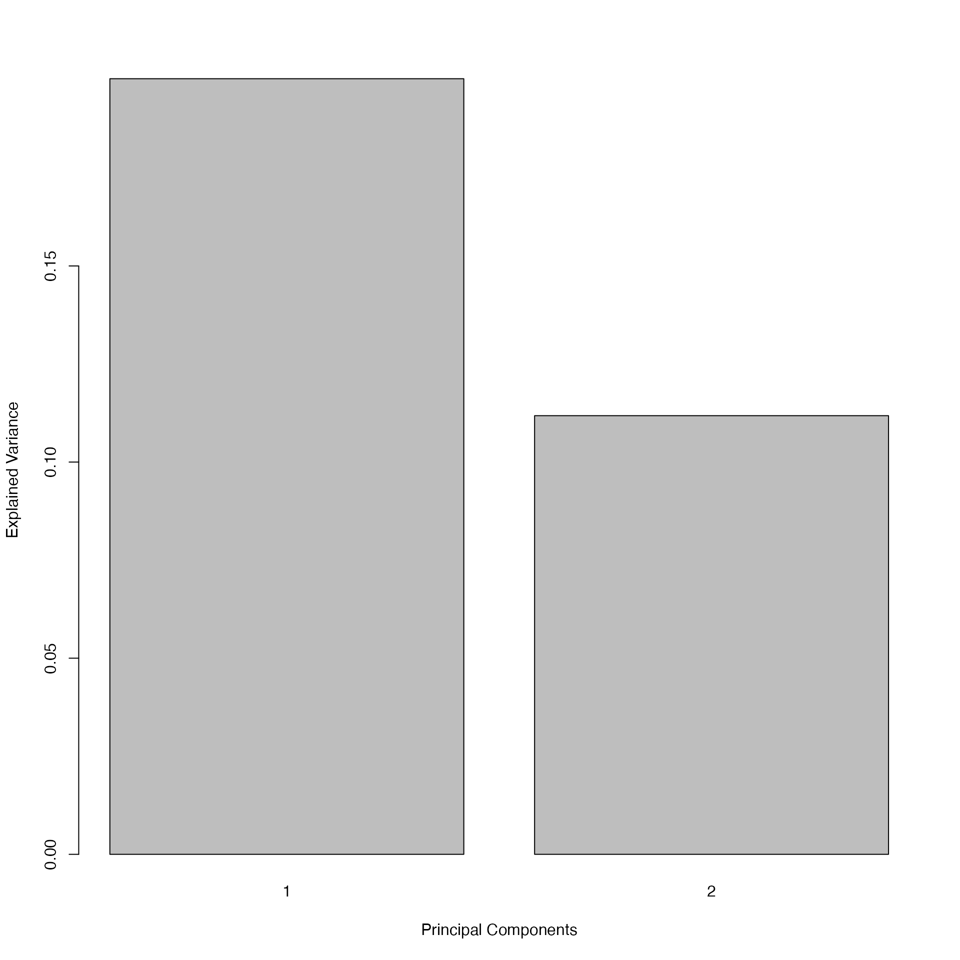
# Two components would be sufficient to explain a moderate proportion of the data's variance
plotIndiv(pca.RCC, group = Y, ind.names = TRUE, # plot the samples projected
          legend = TRUE,
          col.per.group = c("#F68B33", "#388ECC"), # set of colours
          title = 'PCA on the RCC study, comp 1 & 2',
          ellipse = TRUE) # onto the PCA
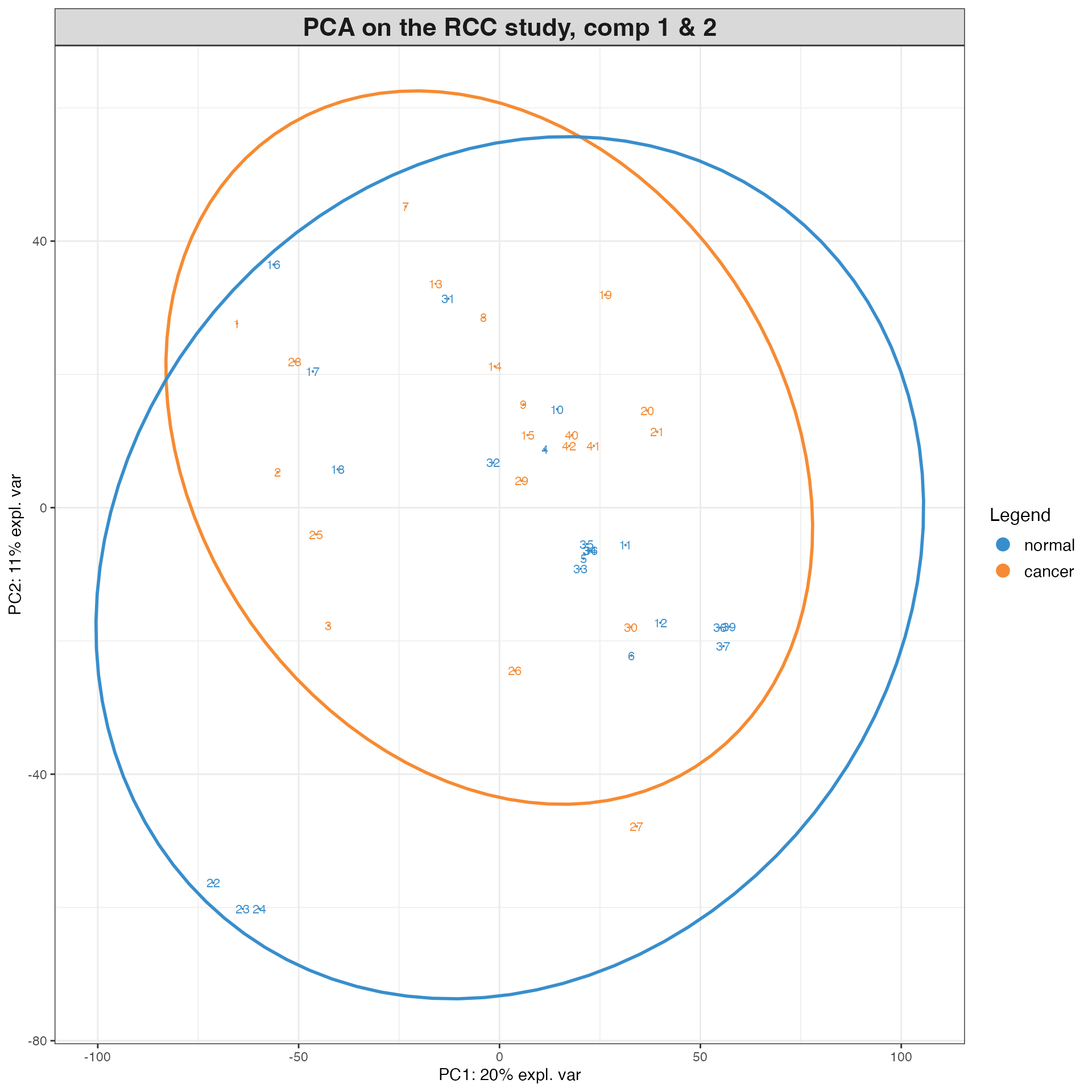
# It seems like only the normal tissue samples are separated from the cancer tissue samples. Cancer tissue samples are heterogenous. This is expected as the normal tissue samples are expected to have different metabolite profiles compared to the cancer tissue samples.
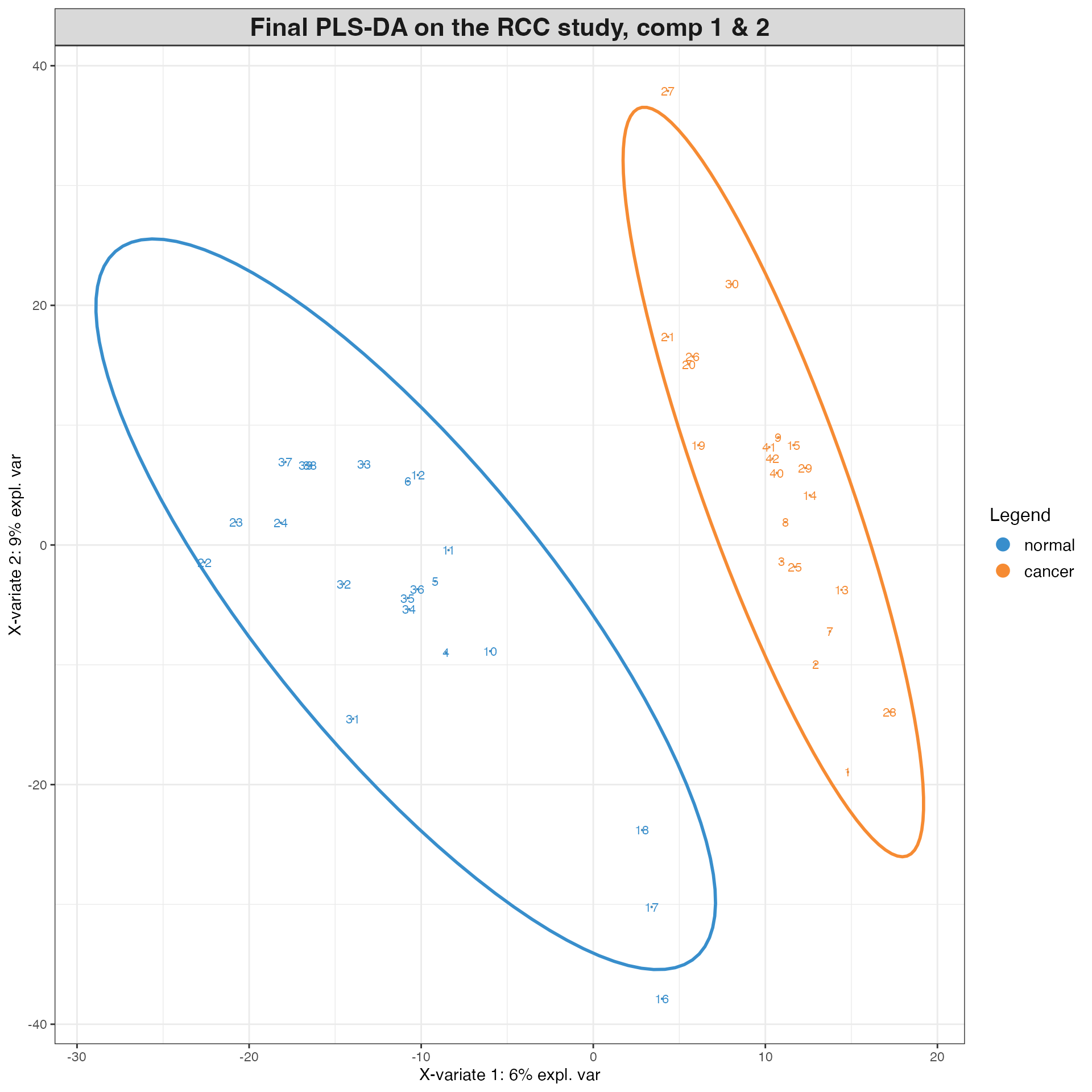
# PLS-DA - Note, PLS-DA is a supervised method, so we need to provide the class labels (Y) to the function. This is designed to find the metabolites that best discriminate between the two classes. Thus, it is not surprising that the PLS-DA model will perform better than the PCA model for class discrimination.
RCC_plsda <- plsda(X, Y, ncomp = 2) # set ncomp to 2 for performance assessment later
# plot the samples projected onto the first two components of the PLS-DA subspace
plotIndiv(RCC_plsda, comp = c(1,2), # plot samples from final model
group = Y, ind.names = TRUE, # colour by class label
ellipse = TRUE, legend = TRUE, # include 95% confidence ellipse,
col.per.group = c("#F68B33", "#388ECC"), # set of colours
title = 'Final PLS-DA on the RCC study, comp 1 & 2')
# list their VIP scores
# Obtain the VIP (Variable Importance in Projection) scores for the fitted PLS-DA model
VIP_scores <- mixOmics::vip(RCC_plsda)

# extract the  VIP scores
VIP_scores = VIP_scores[, 1]
VIP_scores_df = tibble(
    Name = names(VIP_scores),
    VIP_scores = as.numeric(VIP_scores))
VIP_scores_df = VIP_scores_df %>%
    arrange(desc(VIP_scores))
print(VIP_scores_df)
## # A tibble: 2,923 × 2
##    Name                                                               VIP_scores
##    <chr>                                                                   <dbl>
##  1 1-Stearoyl-2-arachidonoyl-sn-glycero-3-phosphoserine                     3.67
##  2 N-Butylacetamide                                                         3.52
##  3 Guanosine                                                                3.28
##  4 12-Hydroxyjasmonate sulfate                                              3.16
##  5 2-Hydroxy-1-(2,4,6-trihydroxyphenyl)-3-(3,4-dihydroxyphenyl)propa…       3.16
##  6 Avenestergenin A1                                                        3.14
##  7 N-Acetyl-L-arginine                                                      3.08
##  8 3-Methylhistamine                                                        3.08
##  9 Lactose                                                                  3.02
## 10 Arctinone A acetate                                                      3.01
## # ℹ 2,913 more rows
# save the VIP scores as a csv file
write.csv(VIP_scores_df, "MSMICA targeted metabolomics analysis/rcc_targeted_MSMICA_HILICpos_metabolites_PLS-DA_VIP_scores.csv", row.names = FALSE)
# Prepare the data for MSMICA untargeted metabolomics analysis ############################################################################################################
# HILIC positive ############################################################################################################
# all MSMICA identified metabolites in HILIC positive and C18 negative #############################
# transpose the table starting at column 13
feature_table_exp_hilicpos_imputed_t = t(feature_table_exp_hilicpos_imputed[,3:ncol(feature_table_exp_hilicpos_imputed)])
feature_table_exp_hilicpos_imputed_t = as.data.frame(feature_table_exp_hilicpos_imputed_t)

# set the column names as the combination of mz and time
colnames(feature_table_exp_hilicpos_imputed_t) = paste0(feature_table_exp_hilicpos_imputed$mz, "_", feature_table_exp_hilicpos_imputed$time)

# add Group_ID as a column
feature_table_exp_hilicpos_imputed_t$Group_ID = rownames(feature_table_exp_hilicpos_imputed_t)

# move Group_ID as the first column
feature_table_exp_hilicpos_imputed_t = tibble(feature_table_exp_hilicpos_imputed_t) %>%
    dplyr::select(Group_ID, everything())

# Seperate the Group_ID into columns: Group, Temperature, Time, SampleID
feature_table_exp_hilicpos_imputed_t = feature_table_exp_hilicpos_imputed_t %>%
    tidyr::separate(Group_ID, c("Group", "Temperature", "Time"), sep = "_") %>%
    # create a new column, sample_tyoe, to indicate the sample type: if Group starts with NM, then it is normal, otherwise it is cancer
    mutate(sample_type = ifelse(stringr::str_detect(Group, "^NM"), "normal", "cancer")) %>%
    # move sample type to the first column
    dplyr::select(sample_type, everything())

# separate the Group column into Group and ParticipantID: the first two characters are Group, the rest are ParticipantID
feature_table_exp_hilicpos_imputed_t = feature_table_exp_hilicpos_imputed_t %>%
    tidyr::separate(Group, c("Group", "ParticipantID"), sep = 2)

# Convert all intensity values to log2
feature_table_exp_hilicpos_imputed_t[, -c(1:5)] = feature_table_exp_hilicpos_imputed_t[, -c(1:5)] %>%
    mutate_all(~log2(.))

# check the data ready for MSMICA untargeted metabolomics analysis
print(feature_table_exp_hilicpos_imputed_t)
## # A tibble: 14 × 2,810
##    sample_type Group ParticipantID Temperature Time  `85.0284_49` `85.0477_83`
##    <chr>       <chr> <chr>         <chr>       <chr>        <dbl>        <dbl>
##  1 normal      NM    11            GS          0             26.4         24.3
##  2 normal      NM    4             GS          0             25.7         23.5
##  3 normal      NM    5             GS          0             26.5         23.6
##  4 normal      NM    6             GS          0             25.5         24.1
##  5 normal      NM    7             GS          0             25.6         22.9
##  6 normal      NM    8             GS          0             26.0         24.0
##  7 normal      NM    9             GS          0             24.6         23.3
##  8 cancer      TM    11            GS          0             26.6         23.6
##  9 cancer      TM    4             GS          0             24.8         23.3
## 10 cancer      TM    5             GS          0             26.6         23.0
## 11 cancer      TM    6             GS          0             26.6         24.6
## 12 cancer      TM    7             GS          0             26.4         24.8
## 13 cancer      TM    8             GS          0             25.7         21.3
## 14 cancer      TM    9             GS          0             25.3         23.8
## # ℹ 2,803 more variables: `85.0841_109` <dbl>, `86.06_86` <dbl>,
## #   `86.0964_48` <dbl>, `86.9086_63` <dbl>, `86.9504_32` <dbl>,
## #   `87.0441_293` <dbl>, `87.0553_86` <dbl>, `87.0619_32` <dbl>,
## #   `87.0917_284` <dbl>, `87.0998_48` <dbl>, `87.174_33` <dbl>,
## #   `87.2858_33` <dbl>, `87.3982_35` <dbl>, `87.5098_35` <dbl>,
## #   `88.0216_281` <dbl>, `88.0393_279` <dbl>, `88.0393_83` <dbl>,
## #   `88.0578_79` <dbl>, `88.0757_86` <dbl>, `88.9526_258` <dbl>, …
# C18 negative ############################################################################################################
# all MSMICA identified metabolites #############################
feature_table_exp_c18neg_imputed_t = t(feature_table_exp_c18neg_imputed[,3:ncol(feature_table_exp_c18neg_imputed)])
feature_table_exp_c18neg_imputed_t = as.data.frame(feature_table_exp_c18neg_imputed_t)

# set the column names as the combination of mz and time
colnames(feature_table_exp_c18neg_imputed_t) = paste0(feature_table_exp_c18neg_imputed$mz, "_", feature_table_exp_c18neg_imputed$time)

# add Group_ID as a column
feature_table_exp_c18neg_imputed_t$Group_ID = rownames(feature_table_exp_c18neg_imputed_t)

# move Group_ID as the first column
feature_table_exp_c18neg_imputed_t = tibble(feature_table_exp_c18neg_imputed_t) %>%
    dplyr::select(Group_ID, everything())

# Seperate the Group_ID into columns: Group, Temperature, Time, SampleID
feature_table_exp_c18neg_imputed_t = feature_table_exp_c18neg_imputed_t %>%
    separate(Group_ID, c("Group", "Temperature", "Time"), sep = "_") %>%
    # create a new column, sample_tyoe, to indicate the sample type: if Group starts with NM, then it is normal, otherwise it is cancer
    mutate(sample_type = ifelse(stringr::str_detect(Group, "^NM"), "normal", "cancer")) %>%
    # move sample type to the first column
    dplyr::select(sample_type, everything())

# separate the Group column into Group and ParticipantID: the first two characters are Group, the rest are ParticipantID
feature_table_exp_c18neg_imputed_t = feature_table_exp_c18neg_imputed_t %>%
    separate(Group, c("Group", "ParticipantID"), sep = 2)

# Convert all intensity values to log2
feature_table_exp_c18neg_imputed_t[, -c(1:5)] = feature_table_exp_c18neg_imputed_t[, -c(1:5)] %>%
    mutate_all(~log2(.))

# check the data ready for MSMICA untargeted metabolomics analysis
print(feature_table_exp_c18neg_imputed_t)
## # A tibble: 14 × 4,220
##    sample_type Group ParticipantID Temperature Time  `85.0044_123` `85.0044_288`
##    <chr>       <chr> <chr>         <chr>       <chr>         <dbl>         <dbl>
##  1 normal      NM    11            GS          0              22.9          22.1
##  2 normal      NM    4             GS          0              23.3          21.9
##  3 normal      NM    5             GS          0              22.0          21.6
##  4 normal      NM    6             GS          0              22.4          21.6
##  5 normal      NM    7             GS          0              23.0          21.9
##  6 normal      NM    8             GS          0              21.1          21.7
##  7 normal      NM    9             GS          0              20.9          21.6
##  8 cancer      TM    11            GS          0              23.7          22.0
##  9 cancer      TM    4             GS          0              19.8          21.8
## 10 cancer      TM    5             GS          0              23.5          22.0
## 11 cancer      TM    6             GS          0              23.5          22.1
## 12 cancer      TM    7             GS          0              23.4          21.8
## 13 cancer      TM    8             GS          0              23.4          21.2
## 14 cancer      TM    9             GS          0              22.6          21.7
## # ℹ 4,213 more variables: `85.0295_293` <dbl>, `85.0295_25` <dbl>,
## #   `85.0295_95` <dbl>, `85.3585_236` <dbl>, `85.7258_217` <dbl>,
## #   `86.0248_292` <dbl>, `86.0248_91` <dbl>, `86.1808_294` <dbl>,
## #   `87.0087_24` <dbl>, `87.02_289` <dbl>, `87.0273_34` <dbl>,
## #   `87.0452_30` <dbl>, `87.4819_227` <dbl>, `87.5205_173` <dbl>,
## #   `87.8345_243` <dbl>, `88.004_198` <dbl>, `88.0404_29` <dbl>,
## #   `88.988_32` <dbl>, `89.0088_23` <dbl>, `89.0194_24` <dbl>, …
############################# limma paired t-test #############################
# HILIC positive ############################################################################################################
# Factorize the samples into normal and cancer
Group_hilicpos = factor(feature_table_exp_hilicpos_imputed_t$sample_type, levels = c("normal", "cancer"))

# Factorize the ParticipantID
ParticipantID_hilicpos = factor(feature_table_exp_hilicpos_imputed_t$ParticipantID)

# Create the design matrix
design_T_hilicpos <- model.matrix(~ ParticipantID_hilicpos+Group_hilicpos)

# Extract the intensity values for the limma analysis
hilicpos_intensity = feature_table_exp_hilicpos_imputed_t[, 6:ncol(feature_table_exp_hilicpos_imputed_t)]
hilicpos_intensity = as.data.frame(hilicpos_intensity)

# transpose the metabolite intensity data
y_T_hilicpos = t(hilicpos_intensity)

# Fit the linear model
fit_hilicpos = lmFit(y_T_hilicpos, design_T_hilicpos)
fit2_hilicpos <- eBayes(fit_hilicpos)

# chcek the top table in the limma paited t-test output
topTable(fit2_hilicpos, coef="Group_hilicposcancer", adjust="BH")
##                  logFC  AveExpr         t     P.Value adj.P.Val         B
## 381.0789_83  -1.294320 25.34860 -4.126351 0.002771802 0.9989403 -4.484285
## 387.0549_178 -1.559068 21.73473 -3.999655 0.003337587 0.9989403 -4.487121
## 242.1749_28  -2.066738 22.05930 -3.806452 0.004449652 0.9989403 -4.491727
## 386.238_27   -2.618954 22.10443 -3.758988 0.004779116 0.9989403 -4.492913
## 559.5185_31  -3.849687 21.31891 -3.624924 0.005856884 0.9989403 -4.496382
## 264.1957_34  -2.832936 22.93908 -3.601827 0.006067149 0.9989403 -4.496998
## 117.1103_42  -3.106604 22.83724 -3.535649 0.006714842 0.9989403 -4.498793
## 465.0513_214  1.757063 22.08679  3.495121 0.007147086 0.9989403 -4.499915
## 442.3889_29   2.453958 22.07238  3.460156 0.007543503 0.9989403 -4.500897
## 599.5033_29  -2.350697 21.55573 -3.441356 0.007766128 0.9989403 -4.501430
# Extract all relevant values from the limma output
limma_outcome_hilicpos = data.frame(
    Cancer_log2FC = c(fit2_hilicpos$coefficients[, "Group_hilicposcancer"]),
    t_statistic = c(fit2_hilicpos$t[, "Group_hilicposcancer"]),
    p = c(fit2_hilicpos$p.value[, "Group_hilicposcancer"]))

limma_outcome_hilicpos$p.fdr = p.adjust(limma_outcome_hilicpos$p, method="BH")
limma_outcome_hilicpos$mz_time = colnames(feature_table_exp_hilicpos_imputed_t[, -c(1:5)])
limma_outcome_hilicpos = tibble(limma_outcome_hilicpos)

# mz, time from feature_table_exp_hilicpos_imputed to limma_outcome_hilicpos
limma_outcome_hilicpos$mz = feature_table_exp_hilicpos_imputed$mz
limma_outcome_hilicpos$time = feature_table_exp_hilicpos_imputed$time

# Organize the column names: mz, time, t_statistics, p, p.fdr, Cancer_log2FC
limma_outcome_hilicpos = limma_outcome_hilicpos %>%
    dplyr::select(mz, time, t_statistic, p, p.fdr, Cancer_log2FC) %>%
    arrange(p) %>%
    tibble()

# select only the significant metabolites
limma_outcome_hilicpos_sig_untargeted = limma_outcome_hilicpos %>%
    filter(p < 0.05)

# left join the MSMICA results to the limma_outcome_hilicpos_sig based on mz and time
limma_outcome_hilicpos_sig_untargeted_MSMICA = left_join(limma_outcome_hilicpos_sig_untargeted, hilicpos_MSMICA_identified_metabolites, by=c("mz"="mz", "time"="time"))

# print the results
print(limma_outcome_hilicpos_sig_untargeted_MSMICA)
## # A tibble: 87 × 77
##       mz  time t_statistic       p p.fdr Cancer_log2FC mz_time     Adduct Name
##    <dbl> <dbl>       <dbl>   <dbl> <dbl>         <dbl> <chr>       <chr>  <chr>
##  1  381.    83       -4.13 0.00277 0.999         -1.29 381.0789_83 M+K    Lacto…
##  2  387.   178       -4.00 0.00334 0.999         -1.56 NA          NA     NA
##  3  242.    28       -3.81 0.00445 0.999         -2.07 242.1749_28 M+H    Valer…
##  4  386.    27       -3.76 0.00478 0.999         -2.62 NA          NA     NA
##  5  560.    31       -3.62 0.00586 0.999         -3.85 NA          NA     NA
##  6  264.    34       -3.60 0.00607 0.999         -2.83 264.1957_34 M+H    Desve…
##  7  117.    42       -3.54 0.00671 0.999         -3.11 NA          NA     NA
##  8  465.   214        3.50 0.00715 0.999          1.76 NA          NA     NA
##  9  442.    29        3.46 0.00754 0.999          2.45 442.3889_29 M+H    Nonad…
## 10  600.    29       -3.44 0.00777 0.999         -2.35 NA          NA     NA
## # ℹ 77 more rows
## # ℹ 68 more variables: identification_type <chr>, identification_method <chr>,
## #   Probability <dbl>, metabolite_within_feature_number <dbl>,
## #   isomer_exist <lgl>, time_predicted <dbl>, time_difference <dbl>,
## #   mean_intensity <dbl>, PubChem_compound_id <dbl>, HMDB_ID <chr>,
## #   KEGG_ID <chr>, LIPID_MAPS_ID <chr>, ChEBI_ID <dbl>, BioCyc_ID <chr>,
## #   DrugBank_ID <chr>, Mono_mass <dbl>, Formula <chr>, Charge <dbl>, …
# save the result as a csv file
write.csv(limma_outcome_hilicpos_sig_untargeted_MSMICA, "MSMICA untargeted metabolomics analysis/rcc_MSMICA_untargeted_hilicpos_metabolites_limma_paired_t_test.csv", row.names = FALSE)

# C18 negative ############################################################################################################
# Factorize the samples into normal and cancer
Group_c18neg = factor(feature_table_exp_c18neg_imputed_t$sample_type, levels = c("normal", "cancer"))

# Factorize the ParticipantID
ParticipantID_c18neg = factor(feature_table_exp_c18neg_imputed_t$ParticipantID)

# Create the design matrix
design_T_c18neg <- model.matrix(~ ParticipantID_c18neg+Group_c18neg)

# Extract the intensity values for the limma analysis
c18neg_intensity = feature_table_exp_c18neg_imputed_t[, 6:ncol(feature_table_exp_c18neg_imputed_t)]

# transpose the metabolite intensity data
y_T_c18neg = t(c18neg_intensity)

# Fit the linear model
fit_c18neg = lmFit(y_T_c18neg, design_T_c18neg)
fit2_c18neg <- eBayes(fit_c18neg)

# chcek the top table in the limma paited t-test output
topTable(fit2_c18neg, coef="Group_c18negcancer", adjust="BH")
##                  logFC  AveExpr         t      P.Value adj.P.Val         B
## 154.9656_21  -2.882124 22.38869 -6.744578 0.0001101287 0.4641923 -4.189543
## 716.5808_263  1.764388 20.59766  4.949691 0.0009376188 0.8898829 -4.247140
## 466.8895_80   2.005374 19.77082  4.868171 0.0010442325 0.8898829 -4.250799
## 868.6075_282  1.696961 20.85049  4.799984 0.0011435091 0.8898829 -4.253949
## 664.8299_69  -1.195280 21.21145 -4.739879 0.0012395136 0.8898829 -4.256797
## 209.0815_31   1.539345 21.68307  4.389639 0.0020037052 0.8898829 -4.274795
## 221.0123_29   1.417734 23.97016  4.069227 0.0031584377 0.8898829 -4.293575
## 403.2516_246  1.681656 22.53564  3.949546 0.0037578698 0.8898829 -4.301216
## 487.0009_61  -1.732563 21.04422 -3.888754 0.0041078412 0.8898829 -4.305236
## 310.283_263   1.594794 23.80621  3.872067 0.0042098608 0.8898829 -4.306356
# Extract all relevant values from the limma output
limma_outcome_c18neg = data.frame(
    Cancer_log2FC = c(fit2_c18neg$coefficients[, "Group_c18negcancer"]),
    t_statistic = c(fit2_c18neg$t[, "Group_c18negcancer"]),
    p = c(fit2_c18neg$p.value[, "Group_c18negcancer"]))

limma_outcome_c18neg$p.fdr = p.adjust(limma_outcome_c18neg$p, method="BH")
limma_outcome_c18neg$mz_time = colnames(feature_table_exp_c18neg_imputed_t[, -c(1:5)])
limma_outcome_c18neg = tibble(limma_outcome_c18neg)

# mz, time from feature_table_exp_c18neg_imputed to limma_outcome_c18neg
limma_outcome_c18neg$mz = feature_table_exp_c18neg_imputed$mz
limma_outcome_c18neg$time = feature_table_exp_c18neg_imputed$time

# Organize the column names: mz, time, t_statistics, p, p.fdr, Cancer_log2FC
limma_outcome_c18neg = limma_outcome_c18neg %>%
    dplyr::select(mz, time, t_statistic, p, p.fdr, Cancer_log2FC) %>%
    arrange(p) %>%
    tibble()

# select only the significant metabolites
limma_outcome_c18neg_sig_untargeted = limma_outcome_c18neg %>%
    filter(p < 0.05)

# left join the MSMICA results to the limma_outcome_c18neg_sig based on mz and time
limma_outcome_c18neg_sig_untargeted_MSMICA = left_join(limma_outcome_c18neg_sig_untargeted, c18neg_MSMICA_identified_metabolites, by=c("mz"="mz", "time"="time"))

# print the results
print(limma_outcome_c18neg_sig_untargeted_MSMICA)
## # A tibble: 208 × 77
##       mz  time t_statistic        p p.fdr Cancer_log2FC mz_time     Adduct Name
##    <dbl> <dbl>       <dbl>    <dbl> <dbl>         <dbl> <chr>       <chr>  <chr>
##  1  155.    21       -6.74 0.000110 0.464         -2.88 NA          NA     NA
##  2  717.   263        4.95 0.000938 0.890          1.76 NA          NA     NA
##  3  467.    80        4.87 0.00104  0.890          2.01 NA          NA     NA
##  4  869.   282        4.80 0.00114  0.890          1.70 868.6075_2… M-H    PS(2…
##  5  665.    69       -4.74 0.00124  0.890         -1.20 NA          NA     NA
##  6  209.    31        4.39 0.00200  0.890          1.54 209.0815_31 M-H    3,5-…
##  7  209.    31        4.39 0.00200  0.890          1.54 209.0815_31 M-H    Phos…
##  8  221.    29        4.07 0.00316  0.890          1.42 NA          NA     NA
##  9  403.   246        3.95 0.00376  0.890          1.68 403.2516_2… M-H    7alp…
## 10  487.    61       -3.89 0.00411  0.890         -1.73 NA          NA     NA
## # ℹ 198 more rows
## # ℹ 68 more variables: identification_type <chr>, identification_method <chr>,
## #   Probability <dbl>, metabolite_within_feature_number <dbl>,
## #   isomer_exist <lgl>, time_predicted <dbl>, time_difference <dbl>,
## #   mean_intensity <dbl>, PubChem_compound_id <dbl>, HMDB_ID <chr>,
## #   KEGG_ID <chr>, LIPID_MAPS_ID <chr>, ChEBI_ID <dbl>, BioCyc_ID <chr>,
## #   DrugBank_ID <chr>, Mono_mass <dbl>, Formula <chr>, Charge <dbl>, …
# save the result as a csv file
write.csv(limma_outcome_c18neg_sig_untargeted_MSMICA, "MSMICA untargeted metabolomics analysis/rcc_MSMICA_untargeted_c18neg_metabolites_limma_paired_t_test.csv", row.names = FALSE)